Temperature measurements

Instrumentation

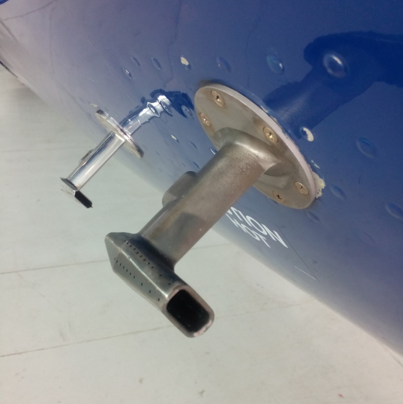
Fig. 1 The de-iced (foreground) and non-de-iced (background) Rosemount Type 102 housings fitted to the FAAM aircraft.

On board the FAAM aircraft, air temperature is measured via internal sensors in two Rosemount Model 102 housings [T. M. Stickney, 1994], one de-iced (configuration B), the other non-de-iced, as shown in Fig. 1. Both housings employ similar inlets to draw flow across the sensing elements, designed to minimise water and particle ingress, as well as minimising interaction of the air with the inlet walls. The housings are designed to, as far as possible, bring the air to rest relative to the aircraft. As the air enters the housings, it slows and is compressed, increasing its temperature. The sensors inside the housings are resistance based thermometers - either platinum resistance thermometers or thermistors. Their resistance is measured using a circuit at the rear core console designed and built in-house. They measure a temperature known as the indicated temperature, \(T_i\), which is higher than the static air temperature outside the aircraft. \(T_i\) is close to the total air temperature (the maximum air temperature which would be attained by complete conversion of the kinetic energy of the air in the housing), \(T_{tot}\). Our measured temperature, \(T_i\), must be converted to the more useful static air temperature, \(T_s\), also known as the true air temperature (parameters TAT_DI_R and TAT_ND_R).

The static air temperature, \(T_s\), is related to the total air temperature by

(6)\[ \frac{T_{tot}}{T_s}=1+\left(\frac{\gamma-1}{2}\right)\times M^2\]

where \(\gamma\) is the ratio of the specific heat capacities. This was taken to be 1.4 in post processing v004, and replaced with \(\frac{c_p}{c_v}\) in post processing v005, calculated using the equations for moist air specific heats given in Khelif et al. (1998), shown here in equations (3) and (4). \(M\) is the Mach number (dry air Mach in v004 and moist Mach in v005) from the RVSM system, described in section Pressure Measurements.

The total temperature is related to the indicated temperature by a recovery factor, as discussed in section Recovery factor.

Indicated temperature: calibration

The original type 102 sensing elements were constructed using a loom of thin platinum wire, as shown in Fig. 2 (left), the resistance of which changes with temperature. These sensors have been used on the aircraft for many years, although several issues with their continued usage have arisen:

• The low thermal mass of the thin platinum wire means that the response of part of these probes to changing air temperature is fast. However the mica support responds more slowly to temperature fluctuations, and as such the probes exhibit two time constants [C. A. Friehe, 1992].

• The fragile platinum wire loom can easily be damaged in-flight, causing long-term probe degredation ranging from calibration drifts over time to complete probe failure, as demonstrated in Fig. 3.

• There is a dwindling stock of these loom-type sensors at FAAM. The manufacturer, now UTC Aerospace, no longer routinely produces these sensors.

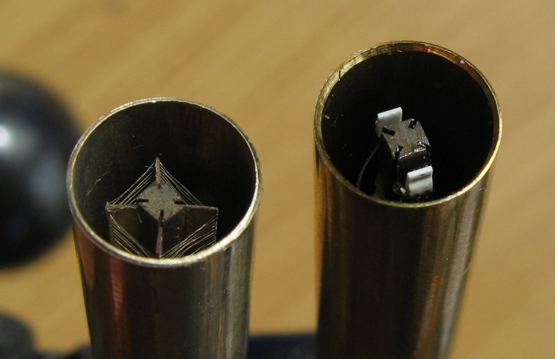
Fig. 2 An original “loom”-type PRT sensor (left) and a modified “plate”-type sensor (right).

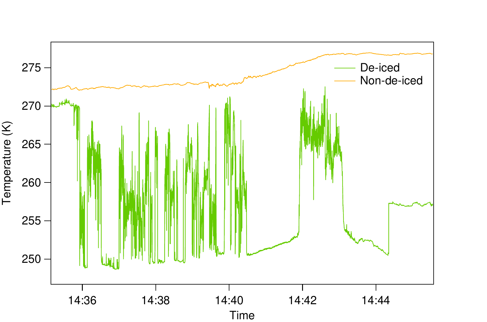
Fig. 3 The final few minutes of flight B944, during which the loom-type PRT sensor in the de-iced housing failed at 14:36. The plate-type sensor in the non-de-iced housing was unaffected.

An alternative solution was developed at FAAM which utilises the existing Rosemount housings but replaces the platinum loom with two thin-film IST MiniSens PT100 platinum resistance thermometers (referred to here as “plate-type”), wired in parallel, shown in Fig. 2 (right). These modified sensors have been shown to be robust and maintain a stable calibration over the course of many months’ flying. The use of two sensing elements, as opposed to one, means that flight data can be recovered if one element fails - a re-calibration of the remaining element is all that is required. When two of these sensors are fitted to the aircraft (one in each housing), they consistently give agreement between the de-iced and non-de-iced temperature measurements better than 0.1 \(^\circ\text{C}\). The drawback to these sensors is their response time. Despite their small size, they still have a greater thermal mass than the thin platinum loom of the original Rosemount sensors and are thus comparatively slow to respond to temperature fluctuations. With time response being equivalent to spatial resolution for an airborne platform, a third option for temperature measurement using thermistors is under development and described in FAAM013005.

There are two stages of calibration involved in producing the indicated temperature measurement: quantifying the relationship between each sensor’s resistance and temperature, and quantifying of the relationship between resistance and ‘counts’ measured on the aircraft data system (known as DECADES).

The resistance, \(R\), to temperature, \(T_i\) calibration is done at the National Physical Laboratory (NPL), after a sensor has been fitted for 30 flights or when drift is suspected. At NPL, sensors are calibrated in a test chamber, in air, and compared with reference PRTs at 10 K intervals between 213 K and 323 K. Each calibration certificate states:

“Traceability of measurement was provided by calibration of the reference thermometers to the International Temperature Scale of 1990 (ITS-90) through NPL Temperature Standard. As requested the PRTs were monitored using a precision resistance bridge with traceability to national standards, using an excitation current of 2.8 mA. At each generated condition a time of not less than 60 minutes was allowed for temperature to equilibrate. A set of 10 readings recorded at 1 minute intervals was then taken from the instruments under test.”

The resulting calibration points are fit using a quadratic curve to produce a parameterisation for \(R\) vs \(T_i\).

At FAAM, we perform calibrations (‘DECADES calibrations’) of the resistance/voltage to ‘counts’ relationship of the relevant channels on the aircraft data system at least once per year. These DECADES calibrations involve replacing temperature sensors with fixed resistors, at 3 \(\Omega\) intervals between 35 and 65 \(\Omega\), and recording the counts at each calibration point for 10 seconds. The resistance of the fixed resistors are measured using a Keithley 197 digital multimeter (DVM), which is regularly calibrated. The resulting calibration points are used to produce a linear fit for counts vs \(R\), which is combined with the quadratic \(R\) vs \(T_i\) to convert from counts to indicated temperature.

Indicated temperature: uncertainty

For the PRT sensors, the combined uncertainty in indicated temperature is calculated by summation in quadrature using a spreadsheet model, as described, for example, in 9.2 of NPL Good Practice Guide No. 11 [Bell, 2001] [1]. Table 1 lists the known sources of uncertainty in indicated temperature, along with the likely probability distribution associated with each source. Where these are uncertainties in resistance or counts, they have been converted to equivalent uncertainties in temperature by applying a typical calibration for a 50 \(\Omega\) PRT.

Table 1 Sources of uncertainty associated with temperature measurements.

Source	Loom	Plate	Distribution	Divisor	Description
Sensor Drift	0.24	0.025	Assumed normal	1	Repeatability of \(R\) to \(T_i\) calibrations. Calculated from the drift between calibrations of the same sensor over years. Greater for looms than for plates.
NPL calibration residual	0.0057	0.013	Assumed normal	1	Uncertainty associated with quadratic fit applied to NPL \(R\) to \(T_i\) calibration. Taken to be the residual standard deviation over all calibration points

Source	DI	NDI	Distribution	Divisor	Description
DECADES cal. variation	0.21	0.12	Assumed normal	1	Repeatability of DECADES calibrations, estimated using the standard deviation across many years of calibrations performed using the same set of resistors
DECADES cal. residual	0.094	0.024	Assumed normal	1	Uncertainty associated with the linear fit applied to the DECADES calibration. Taken to be the residual standard deviation over all calibration points
Noise with fixed resistor	0.0030	0.0028	Assumed normal	1	Noise recorded when fixed resistor fitted to the aircraft in place of sensing element.

Source	All	Distribution	Divisor	Description
Keithley DVM calibration	0.04	Assumed normal	1	Uncertainty associated with calibration of digital multimeter, provided on its calibration certificate.
Keithley DVM stability	0.02	Assumed normal	1	Temperature stability of digital multimeter, provided on specifications sheet.
Keithley DVM resolution uncertainty	0.0025	Rectangular	\(\sqrt{3}\)	Resolution of digilal multimeter
NPL resistance measurement	0.0025	Rectangular	\(\sqrt{3}\)	Half the final quoted digit in resistance measurements supplied on NPL calibration certificates
DECADES resolution uncertainty	0.00004	Rectangluar	\(\sqrt{3}\)	Resolution of the aircraft data acquisition system, i.e. K per DECADES count.

Source	T dependent	Distribution	Divisor	Description
NPL calibration uncertainty	0.04	Assumed normal	1	Provided on the NPL calibration certificate, varies with indicated temperature

Recovery factor

Due to the inability to reach complete adiabatic compression within the Rosemount housings, the temperature indicated by the sensors, \(T_i\), is less than \(T_{tot}\). To account for this, a recovery factor is required. Rosemount state in Technical Report 5755 [T. M. Stickney, 1994] that their Type 102 sensors exhibit a variable recovery factor below a Mach number of 1. They define this variable recovery factor as

(7)\[ \eta=\frac{T_{tot}-T_i}{T_{tot}}\]

and provide plots of \(\eta\) vs Mach number based on wind tunnel measurements. The values of \(\eta\) provided in the report for the de-iced housing (Model 102 configuration B) are applicable to fully encased platinum resistance thermometers, hermetically sealed in the wall of a platinum shell with a radiation shield, which are not used at FAAM. For the non-de-iced housing, \(\eta\) values are provided for an open wire element - the platinum loom-type sensors originally used at FAAM. The report states that when an open wire sensor is used in either configuration of the de-iced housing, performance will be “comparable”, yet no data is provided. This lack of information about how \(\eta\) varies with Mach in the de-iced housing has led to the recovery factors for both housings being determined using flight data.

Constant recovery factor, \(r\) (v004)

(See p_rio_temps.py [FAAM, n.d.])

Attempts have been made in the past to measure a constant recovery factor, \(r\), on the FAAM aircraft, defined as

\[r=\frac{T_i-T_s}{T_{tot}-T_s}\]

Assuming a constant adiabatic recovery factor,

(8)\[ \frac{T_i}{T_s}=1+\left(r\times\frac{\gamma-1}{2}\times M^2\right)\]

By flying at different speeds through air of constant temperature, plots of \(T_i\) vs \(M^2\) can be obtained. (8) can be rearranged to

(9)\[ T_i=T_s+rT_s\left(\frac{\gamma-1}{2}\right)M^2\]

The gradient and y-intercept of a linear fit to \(T_i\) vs \(M^2\) allows \(r\) to be determined for each housing. Unfortunately, the resulting values of \(r\) are variable, possibly due to small changes in static air temperature during measurements or errors in the measurement of the static and dynamic pressure. Nevertheless, values of \(r\) calculated from this analysis (0.9928 for the de-iced housing and 0.999 for the non-de-iced housing) were used in v004 of the post processing. The agreement between the de-iced and the non-de-iced static air temperatures calculated using these constant recovery factors is better than when calculated using the variable recovery factors given in the Rosemount report. However, agreement between the two housings does not necessarily mean that either measurement is accurate.

Variable recovery factor, \(\eta\) (v005)

(See p_recovery_factor.py [FAAM, n.d.] and p_prt_temps.py [FAAM, n.d.])

Discussions with Collins Aerospace in December 2020 confirmed that the Rosemount 5755 report [T. M. Stickney, 1994] contains reliable data for the recovery factor of open-wire sensors in the non-de-iced housing, but does not contain that data for the de-iced housing. This information, combined with the fact that a new, low-noise circuit for measuring the resistances of the temperature sensors was installed in December 2017, means that we can now estimate the variable recovery factor for the de-iced housing based on the assumption that the non-de-iced recovery factor provided in the Rosemount 5755 report is correct. The following describes the analysis implemented in deiced_recovery_factor_prt_only_2021.py [Price, n.d.].

Following on from equations (6) and (7),

(10)\[ \frac{T_i}{T_s}=(1-\eta)\left(1+\frac{\gamma-1}{2}\times M^2\right)\]

The static temperature, \(T_s\) measured by both housings should be the same:

\[\frac{T_{i,n}}{(1-\eta_n)\left(1+\frac{\gamma-1}{2}\times M^2\right)}=\frac{T_{i,d}}{(1-\eta_d)\left(1+\frac{\gamma-1}{2}\times M^2\right)}\]

The \(M^2\) terms cancel, and rearranging:

\[\eta_d=1-\frac{T_{i,n}}{T_{i,d}}\left(1-\eta_n\right)\]

For the Mach range of the FAAM aircraft (0.2 to 0.7), the data shown in Figure 20 in the Rosemount 5755 report can be described by:

\[\eta_n=-6.0943146 \times 10^{-4} M^2 + 1.4054157 \times 10^{-3} M\]

(11)\[ \sigma_{\eta_n}=-3.4581190 \times 10^{-4} M^2 + 5.9345748 \times 10^{-4} M\]

(\(\sigma_n\) is calculated from the error band shown in Figure 20 of the Rosemount 5755 report, confirmed by Collins Aerospace to represent the 2:math:sigma uncertainty).

Using flight data for the ratio of the indicated temperatures, \(\frac{T_{i,n}}{T_{i,d}}\), we can calculate thousands of “measurements” of \(\eta_d\) across a range of Mach. The analysis was restricted to cloud-free, straight and level runs. To achieve this, the data was filtered so that measurements collected under the following conditions were removed:

• profiles up or down (filtered by assessing angle of attack and successive changes in static pressure)

• possibility of cloud (difference between the static temperature and the dewpoint measured by the General Eastern chilled mirror hygrometer less than 2 K)

• on the ground

• magnitude of the roll greater than 0.5 degree

• angle of attack greater than 8 degrees or less than 3 degrees

• large difference (greater than 1 K) between the two static air temperatures calculated using the standard constant recovery factors (this is to filter out instances of sensor damage or poor calibration)

Initial analysis was performed for flights between December 2017 and March 2020 where a PRT sensor (either “loom”, the original wound wire sensors from Rosemount, or “plate”, a modified version using a commercially sourced thin film PRT) was fitted in both housings. A small minority of flights are excluded due to issues with sensors, leaving a total of 49 flights. Fig. 4 shows each measurement of the ratio of the indicated temperatures, as a function of Mach number. No strong dependency of the ratio on Mach number is observed, so \(\eta_d\) is calculated using the average ratio, \(\alpha\), such that

\[\eta_d=1-\alpha\left(1-\eta_n\right)\]

The uncertainty in the variable recovery factor calculated for the de-iced housing is therefore:

(12)\[\sigma_{\eta_d}^2=\left(\eta_n-1\right)^2\sigma_{\alpha}^2 + \alpha^2\sigma_{\eta_n}^2\]

The resulting values of the mean ratio, \(\alpha\), and its standard deviation, \(\sigma_{\alpha}\) are as follows:

\[\begin{split}\alpha &= 0.9989 \\ \sigma_{\alpha} &= 0.0006\end{split}\]

Fig. 5 shows each calculated value of \(\eta_d\) as a grey datapoint, along with a dashed red line showing \(\eta_d\) calculated using the average ratio of indicated temperatures (i.e. using equations 10 and 12, with the value of \(\alpha\) given in 14). Fig. 6 shows a histogram of the differences between the true air temperatures calculated for each housing (de-iced true air temperature \(-\) non-de-iced true air temperature). It can be seen that changing from the old constant recovery factors, \(r_d\) and \(r_n\), to the new variable recovery factors, \(\eta_d\) and \(\eta_n\), we reduce the mean difference between our two true air temperature measurements by 0.225 K. The change from using \(r\) to \(\eta\) increases the non-de-iced true air temperature by around 0.1 K, and increases the de-iced true air temperature by around 0.3 K.

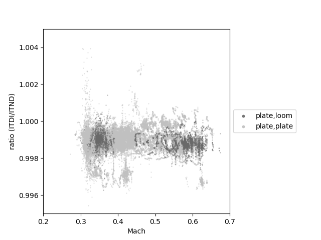
Fig. 4 The ratio, \(\frac{T_{i,n}}{T_{i,d}}\), of indicated temperatures, vs Mach, for flights for which a PRT was fitted in each housing. A plate-type sensor was always fitted in the de-iced housing. Light grey points come from flights when a plate-type sensor was also fitted in the non-de-iced housing; dark grey points comes from flights where a loom-type sensor was fitted in the non-de-iced housing. Data shown is collected using a variety of individual sensors - two different looms, and six different PRTs, resulting in a total of six configurations.

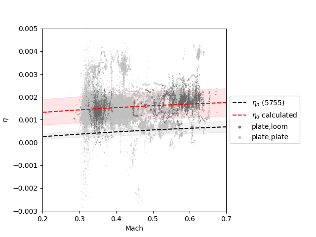
Fig. 5 Calculated values of \(\eta_d\) for flights when a plate-type sensor was fitted in the de-iced housing and a loom-type sensor was fitted in the non-de-iced housing (dark grey points) and flights when a plate-type sensor was fitted in both housings (light grey points). Overlaid as a dashed red line is the curve of \(\eta_d\) calculated using the average ratio of indicated temperatures, \(\alpha\). The black dashed line is a reproduction of the line given in Figure 20 of Rosemount report 5755 for the variable recovery factor of the non-de-iced housing. Uncertainty bands represent the \(1 \sigma\) uncertainty for each \(\eta\).

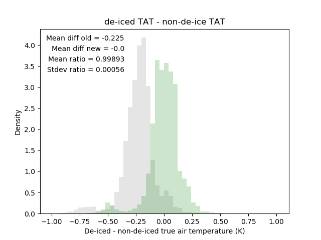
Fig. 6 Histograms to show the difference between the true (static) air temperature (TAT or \(T_s\)) measurements in each housing, for flights where a PRT was fitted in each housing. Data calculated using the fixed recovery factors is shown in grey; the same calculated using the new variable recovery factors is shown in green.

In summary, the variable recovery factor for the non-de-iced housing provided in Rosemount 5755 is implemented in v005 of the post processing, along with the variable recovery factor calculated here for the de-iced housing, based on flights where a PRT is fitted in both housings:

\[\eta_n=-6.0943146 \times 10^{-4} M^2 + 1.4054157 \times 10^{-3} M\]

\[\sigma_{\eta_n}=-3.4581190 \times 10^{-4} M^2 + 5.9345748 \times 10^{-4} M\]

\[\eta_d=1-\alpha\left(1-\eta_n\right)\]

\[\sigma_{\eta_d}^2=\left(\eta_n-1\right)^2\sigma_{\alpha}^2 + \alpha^2\sigma_{\eta_n}^2\]

with \(\alpha=0.9989\) and \(\sigma_{\alpha}=0.0006\).

The uncertainty in \(\eta_n\) due to any uncertainty in Mach is negligible in comparison with the uncertainty given in Rosemount Report 5755 [T. M. Stickney, 1994]. Since \(\eta_d\) is empirically determined using Mach on our aircraft, and the most significant source of uncertainty in Mach is the position error (and will therefore not vary between the measurements made in the determination of \(\eta_d\) and measurements made in general), the uncertainty in \(\eta_d\) due to uncertainty in Mach is also considered to be negligible, and comes from the uncertainty in \(\eta_n\) and the uncertainty relating to the empirical determination.

Further work on recovery factors will include:

• A further assessment of any Mach dependence in the ratio of indicated temperatures, and thus the validity of using \(\alpha\). There may be a hint of a decrease in the ratio at high Mach number.

• Expanding the analysis to thermistor sensors.

• Collecting more data for at high altitude, especially with a loom-type PRT fitted in the de-iced housing.

Combined uncertainty in static air temperature

(See p_prt_uncertainties.py [FAAM, n.d.])

Finding the uncertainty in static air temperature, \(u(T_s)\) (reported in the core file as parameters TAT_ND_R_CU and TAT_DI_R_CU), requires combining the uncertainties in indicated temperature, \(T_i\), of the sensor, the Mach number, \(M\), the ratio of specific heats, \(\gamma\), and the recovery factor, \(\eta\) (no uncertainty in recovery factor \(r\) is available). The combined uncertainty in \(T_s\) is calculated according to the law of propagation of uncertainty as defined in section 5 of the ISO/IEC Guide to the Expression of Uncertainty in Measurement [ISO/IEC, 2008]:

(13)\[u^2(T_s)= \left(\frac{\partial T_s}{\partial T_i}\right)^2u^2(T_i) + \left(\frac{\partial T_s}{\partial \eta}\right)^2u^2(\eta) + \left(\frac{\partial T_s}{\partial M}\right)^2u^2(M) + \left(\frac{\partial T_s}{\partial \gamma}\right)^2u^2(\gamma)\]

\(u(T_i)\) is calculated using the summation in quadrature of the sources of uncertainty listed in Table 1, for the relevant configuration. \(u(M)\) is given by equation (5). \(u(\eta)\) is given by either equation (11) or (12). Although \(\eta\) is Mach-dependent, given the inherent uncertainty in both \(\eta_n\) and \(\eta_d\) are significantly larger than any uncertainty that would be introduced because of an error in Mach, and given the empirical nature of the method used to determine \(\eta_d\) for our aircraft, we neglect an contribution to the uncertainty in \(\eta\) from the uncertainty in Mach. The uncertainty in \(\gamma\) resulting from the uncertainty in the volume mixing ratio measurement from the WVSS-II (see section Water Vapour Measurements) was calculated by propagation of uncertainties through equations (3) and (4). The resulting uncertainty can be approximated as follows:

\[u(\gamma)=9.4264\cdot10^{-17}w^3 - 3.7152\cdot10^{-12}w^2 + 5.6828\cdot10^{-8}w + 6.3904\cdot10^{-5}\]

where \(w\) is the water vapour volume mixing ratio in ppm.

Fig. 7 shows the relative contributions of each term in equation (13): it can be seen that the terms associated with uncertainty in \(T_i\) and \(M\) are the largest, with the uncertainty in \(\eta\) smaller but still significant. The contribution from the uncertainty associated with \(\gamma\) is negligible.

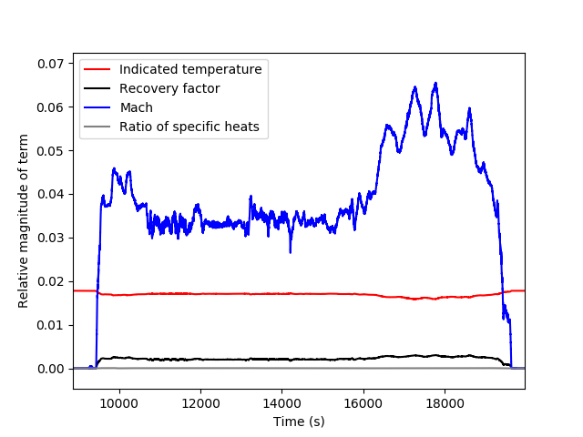
Fig. 7 Relative contibutions of each term in equation (13) over the course of a flight.

Performance in cloud

Both types of Rosemount Model 102 housings can be affected by liquid water and icing, introducing errors in the reported true air temperature which are not included in the uncertainty calculations described above. Liquid water on a sensing element can change its temperature, as can the effect of evaporative cooling. In icing conditions, the housings can clog with ice, meaning that there is little airflow and thus the sensors do not measure the true air temperature. The non-de-iced housing is less susceptible to liquid water ingress than the de-iced housing, whilst the de-iced housing is less susceptible to being clogged with ice. The effect of water or ice is only evident by comparing data from sensors in the two housings: where they agree, the data is likely to be good, but where they disagree it is often impossible to say which, if either, is reading the correct temperature.

Future work

The uncertainty in static air temperature can be reduced most significantly by reducing the uncertainty and correcting the systematic position error which affects the static and dynamic pressures. The next biggest improvement will be in improving the DECADES calibration by using a highly accurate, self-adjusting programmable resistance box (recently purchased). Uncertainty quantification for the thermistor sensors using a Monte Carlo-type method is required, once a new PCB has been finalised.

Footnotes

[1]

For the thermistors, due to the complexity of the self-heating analysis(described in FAAM013005), a Monte Carlo-type analysis will be performed.